Effective exploratory data analysis (EDA) is crucial to most any data science project. For a great first look at how to do EDA in R, check out the 7th chapter of R for Data Science. This post here will point you towards some useful tools to make some aspects of EDA easier and faster.
Prepared to be primed
Over the past few months I have found myself using a few packages or functions over and over again whenever I get my hands on a new dataset. I also have recently stumbled upon some new beauties that I think are worth sharing. This post is meant to be more of a primer than a real deep dive into any one package. Links to learn more about each package/function are included throughout.
# if needed:
# install.packages(c("tidyverse", "janitor", "DataExplorer", "skimr", "trelliscopejs", "gapminder"))

library(tidyverse) # (dplyr, ggplot2, %>%)
library(janitor)
library(DataExplorer)
library(skimr)
library(trelliscopejs)
library(gapminder)

dat <- ggplot2::diamonds
# learn more about diamonds dataset: ?diamonds
An oldie but a goodie
- dplyr::glimpse()
When I first look at a new dataset, I really just want to take a peak, or a glimpse of the data. glimpse from dplyr is perfect for just that. It shows you all the basics of your dataset: number of rows and columns, names and types of variables, and the first several values in each row.
glimpse(dat)
Rows: 53,940
Columns: 10
$ carat   <dbl> 0.23, 0.21, 0.23, 0.29, 0.31, 0.24, 0.24, 0.26, 0...
$ cut     <ord> Ideal, Premium, Good, Premium, Good, Very Good, V...
$ color   <ord> E, E, E, I, J, J, I, H, E, H, J, J, F, J, E, E, I...
$ clarity <ord> SI2, SI1, VS1, VS2, SI2, VVS2, VVS1, SI1, VS2, VS...
$ depth   <dbl> 61.5, 59.8, 56.9, 62.4, 63.3, 62.8, 62.3, 61.9, 6...
$ table   <dbl> 55, 61, 65, 58, 58, 57, 57, 55, 61, 61, 55, 56, 6...
$ price   <int> 326, 326, 327, 334, 335, 336, 336, 337, 337, 338,...
$ x       <dbl> 3.95, 3.89, 4.05, 4.20, 4.34, 3.94, 3.95, 4.07, 3...
$ y       <dbl> 3.98, 3.84, 4.07, 4.23, 4.35, 3.96, 3.98, 4.11, 3...
$ z       <dbl> 2.43, 2.31, 2.31, 2.63, 2.75, 2.48, 2.47, 2.53, 2...
I prefer glimpse over head because glimpse simply gives you more information. Also, when working in an R script, using glimpse is often nicer than using View because View takes you out of the script and can slightly distrupt your flow. I have also had View crash R when being used on very large datasets.
glimpse also works great with the pipe %>%. I like to use it at the end of a series of manipulations on data as a sort of sanity check.
# random dplyr code
dat %>%
    rename(length = x, width = y) %>%
    mutate(price_euro = price * .91) %>%
    filter(carat > .7) %>%
    select(carat, cut, price_euro) %>% glimpse()
Rows: 26,778
Columns: 3
$ carat      <dbl> 0.86, 0.71, 0.78, 0.96, 0.73, 0.80, 0.75, 0.75...
$ cut        <ord> Fair, Very Good, Very Good, Fair, Very Good, P...
$ price_euro <dbl> 2508.87, 2510.69, 2510.69, 2510.69, 2511.60, 2...
snake_case_is_the_best
- janitor::clean_names()
The clean_names() function from the janitor package is awesome for cleaning up annoying column names. You just pipe in your data and it magically converts your columns to snake case. There are other options, too. ?clean_names. Okay maybe this function doesn’t really have much to do with EDA, but quickly standardizing all of your column names sure makes working with them easier.
dat_ugly_names <- tribble(
    ~"BAD Column", ~"Good name?", ~"This-hurts_Me",
    "a",            1,              "fruit",
    "b",            2,              "taco",
    "c",            3,              "corona virus"
)

dat_ugly_names %>% clean_names()
# A tibble: 3 x 3
  bad_column good_name this_hurts_me
  <chr>          <dbl> <chr>
1 a                  1 fruit
2 b                  2 taco
3 c                  3 corona virus
# I use clean_names just about every time I import data from somewhere!
# import dataset from the wild:
# dat <- read_csv("some-crazy-data-from-the-wild.csv) %>% clean_names()
# oh wow, now this wild dataset at least has some tame column names
Data the Explora-data
I am not proud of that subheading. Enter the DataExplorer package to redeem myself. This is a package I plan on diving deeper into myself. Lots of golden nuggets here. From this package, I have used plot_histogram and plot_bar for quite a while. Just this last week (at the time of writing this) I learned about profile_missing and create_report. Finally, while writing this post, I learned about another useful function called introduce.
introduce and profile_missing just take data as an argument, while the other functions allow you to customize the outputs a bit more if desired.
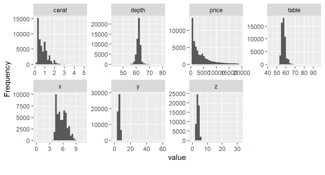
- plot_histogram() - Creates histograms for all continuous variables in a dataset.
dat %>% plot_histogram()
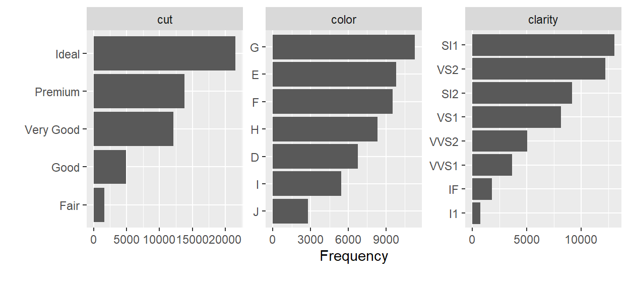
- plot_bar() - Creates bar charts for all discrete variables in a dataset.
dat %>% plot_bar()
- profile_missing() - Tells you the number and percentage of
NAvalues from each of the columns in a dataset.
datasets::airquality %>% profile_missing() # datasets from base R
  feature num_missing pct_missing
1   Ozone          37  0.24183007
2 Solar.R           7  0.04575163
3    Wind           0  0.00000000
4    Temp           0  0.00000000
5   Month           0  0.00000000
6     Day           0  0.00000000
create_report() - Compiles a whole bunch of data profiling statistics (including outputs from the three above functions, correlation between variables, etc.) into an html report. It looks like you can customize it a bunch, but the default report has been sufficient for me (except for setting a y so that a response variable can be included in some of the plotting functions). I won’t include an example here because it produces an html document, but you could probably run
create_report(mtcars)or something in your console to see what it outputs. Lots of good stuff here.introduce() - Describes basic info about the data.
dat %>% introduce()
# A tibble: 1 x 9
   rows columns discrete_columns continuous_colu~ all_missing_col~
  <int>   <int>            <int>            <int>            <int>
1 53940      10                3                7                0
# ... with 4 more variables: total_missing_values <int>,
#   complete_rows <int>, total_observations <int>, memory_usage <dbl>
Hmm. Seeing how the output is formatted, I don’t like it as much. Too wide. I think I would rather use it in combination with glimpse.
dat %>% introduce() %>% glimpse()
Rows: 1
Columns: 9
$ rows                 <int> 53940
$ columns              <int> 10
$ discrete_columns     <int> 3
$ continuous_columns   <int> 7
$ all_missing_columns  <int> 0
$ total_missing_values <int> 0
$ complete_rows        <int> 53940
$ total_observations   <int> 539400
$ memory_usage         <dbl> 3457760
Skim a bit right off the top
- skimr::skim()
From the skimr package, “skim() is an alternative to summary(), quickly providing a broad overview of a data frame.” Now that I use functions from DataExplorer a lot, I don’t use skim as much, but some people might like it.
skim(iris)
| Name | iris |
| Number of rows | 150 |
| Number of columns | 5 |
| _______________________ | |
| Column type frequency: | |
| factor | 1 |
| numeric | 4 |
| ________________________ | |
| Group variables | None |
Variable type: factor
| skim_variable | n_missing | complete_rate | ordered | n_unique | top_counts |
|---|---|---|---|---|---|
| Species | 0 | 1 | FALSE | 3 | set: 50, ver: 50, vir: 50 |
Variable type: numeric
| skim_variable | n_missing | complete_rate | mean | sd | p0 | p25 | p50 | p75 | p100 | hist |
|---|---|---|---|---|---|---|---|---|---|---|
| Sepal.Length | 0 | 1 | 5.84 | 0.83 | 4.3 | 5.1 | 5.80 | 6.4 | 7.9 | ▆▇▇▅▂ |
| Sepal.Width | 0 | 1 | 3.06 | 0.44 | 2.0 | 2.8 | 3.00 | 3.3 | 4.4 | ▁▆▇▂▁ |
| Petal.Length | 0 | 1 | 3.76 | 1.77 | 1.0 | 1.6 | 4.35 | 5.1 | 6.9 | ▇▁▆▇▂ |
| Petal.Width | 0 | 1 | 1.20 | 0.76 | 0.1 | 0.3 | 1.30 | 1.8 | 2.5 | ▇▁▇▅▃ |
You could also pipe this into summary.
| Name | iris |
| Number of rows | 150 |
| Number of columns | 5 |
| _______________________ | |
| Column type frequency: | |
| factor | 1 |
| numeric | 4 |
| ________________________ | |
| Group variables | None |
Honorable mention
- trelliscopejs::facet_trelliscope
Wow, just wow. Go here to check out how to use facet_trelliscope. This function combines the awesomeness of faceting in ggplot2 with the additional interactive power of javascript. I will definitely be exploring trelliscopejs some more. I love what people come up with.
Conclusion
I hope some of this has been useful to you. Most of the functions I mentioned can probably help get you started with EDA. They are especially useful when you take an initial look at a dataset, and perhaps you could continue to use some of these functions during the EDA process. However, simple functions like these do not replace best practices that you have been taught. Hopefully they just support you in whatever your process looks like.
Again, I would point you towards R for Data Science to learn more about EDA in R, and also the 4th chapter of Feature Engineering and Selection for EDA that is more focused on building models.
Thank you so much for reading my first post! Feel free to share this with anyone who might find it helpful or leave a comment pointing towards other useful packages.